Ore Mining Analysis

Written on April 14th, 2023 by Frank Hsiung

Data Source

This is an open dataset about ore mining process public on Kaggle community by a single source provider. The contents are basically describing the factors that are used in floating plant to purify the iron ore flow by removing the impurity(silica). For details of the description, visit: Ore mining

Objectives

The main goal is to use this data to predict how much impurity is in the ore concentrate. As this impurity is measured every hour, if we can predict how much silica (impurity) is in the ore concentrate, we can help the engineers, giving them early information to take actions (empowering!). Hence, they will be able to take corrective actions in advance (reduce impurity, if it is the case) and also help the environment (reducing the amount of ore that goes to tailings as you reduce silica in the ore concentrate).

Data workflow

Here’s some of the outlining features I add for this project:

Memory Saving
Timeseries Data Integrity
Exploratory Data Analysis(EDA)
ML model(LightGBM)

Memory Saving

At first, this notebook was implement and experimented on kaggle for it’s data origin and compatibility of swift testing and play around for ore mining data. Therefore, it is essential to save more memory for larger dataset, one for potential insufficiency of data RAM, another for faster process speed on publish stage on Kaggle.

def reduce_mem_usage(df, verbose=True):
    numerics = ['int16', 'int32', 'int64', 'float16', 'float32', 'float64']
    start_mem = df.memory_usage().sum() / 1024**2    
    for col in df.columns:
        col_type = df[col].dtypes
        if col_type in numerics:
            c_min = df[col].min()
            c_max = df[col].max()
            if str(col_type)[:3] == 'int':
                if c_min > np.iinfo(np.int8).min and c_max < np.iinfo(np.int8).max:
                    df[col] = df[col].astype(np.int8)
                elif c_min > np.iinfo(np.int16).min and c_max < np.iinfo(np.int16).max:
                       df[col] = df[col].astype(np.int16)
                elif c_min > np.iinfo(np.int32).min and c_max < np.iinfo(np.int32).max:
                    df[col] = df[col].astype(np.int32)
                elif c_min > np.iinfo(np.int64).min and c_max < np.iinfo(np.int64).max:
                    df[col] = df[col].astype(np.int64)  
            else:
                if c_min > np.finfo(np.float16).min and c_max < np.finfo(np.float16).max:
                    df[col] = df[col].astype(np.float32)
                elif c_min > np.finfo(np.float32).min and c_max < np.finfo(np.float32).max:
                    df[col] = df[col].astype(np.float32)
                else:
                    df[col] = df[col].astype(np.float64)    
    end_mem = df.memory_usage().sum() / 1024**2
    if verbose: print('Mem. usage decreased to {:5.2f} Mb ({:.1f}% reduction)'.format(end_mem, 100 * (start_mem - end_mem) / start_mem))
    return df

df = pd.read_csv('/kaggle/input/quality-prediction-in-a-mining-process/MiningProcess_Flotation_Plant_Database.csv',decimal=",",parse_dates=["date"],infer_datetime_format=True)
df = reduce_mem_usage(df)

Mem. usage decreased to 70.33 Mb (47.9% reduction)

Features outline

df.head()

	date	%_Iron_Feed	%_Silica_Feed	Starch_Flow	Amina_Flow	Ore_Pulp_Flow	Ore_Pulp_pH	Ore_Pulp_Density	Flotation_Column_01_Air_Flow	Flotation_Column_02_Air_Flow	Flotation_Column_03_Air_Flow	Flotation_Column_04_Air_Flow	Flotation_Column_05_Air_Flow	Flotation_Column_06_Air_Flow	Flotation_Column_07_Air_Flow	Flotation_Column_01_Level	Flotation_Column_02_Level	Flotation_Column_03_Level	Flotation_Column_04_Level	Flotation_Column_05_Level	Flotation_Column_06_Level	Flotation_Column_07_Level	%_Iron_Concentrate	%_Silica_Concentrate
0	2017-03-10 01:00:00	55.200001	16.98	3019.530029	557.434021	395.713013	10.0664	1.74	249.214005	253.235001	250.576004	295.096008	306.399994	250.225006	250.884003	457.395996	432.962006	424.954010	443.558014	502.255005	446.369995	523.343994	66.910004	1.31
1	2017-03-10 01:00:00	55.200001	16.98	3024.409912	563.965027	397.382996	10.0672	1.74	249.718994	250.531998	250.862000	295.096008	306.399994	250.136993	248.994003	451.890991	429.559998	432.938995	448.085999	496.363007	445.921997	498.075012	66.910004	1.31
2	2017-03-10 01:00:00	55.200001	16.98	3043.459961	568.054016	399.667999	10.0680	1.74	249.740997	247.873993	250.313004	295.096008	306.399994	251.345001	248.070999	451.239990	468.927002	434.609985	449.687988	484.411011	447.825989	458.566986	66.910004	1.31
3	2017-03-10 01:00:00	55.200001	16.98	3047.360107	568.664978	397.938995	10.0689	1.74	249.917007	254.487000	250.048996	295.096008	306.399994	250.421997	251.147003	452.441010	458.165009	442.864990	446.209991	471.411011	437.690002	427.669006	66.910004	1.31
4	2017-03-10 01:00:00	55.200001	16.98	3033.689941	558.166992	400.253998	10.0697	1.74	250.203003	252.136002	249.895004	295.096008	306.399994	249.983002	248.927994	452.441010	452.899994	450.523010	453.670013	462.597992	443.682007	425.678986	66.910004	1.31

Goal is to predict % Silica Concentrate
Silica Concentrate is the impurity in the iron ore which needs to be removed
The value of modeling on this target value is that it takes at least an hour to measure the impurity

Timeseries Data Integrity

For this task, there’s an obvious need to treat the data as timeseries format for it’s time continuity and the need mentioned in objectives that we would like to predict the trend and future purity based on current state.

# Set datetime column as index
dt_df = df.set_index('date')

# Pick out discontinuity in data
all_hours = pd.Series(data=pd.date_range(start=dt_df.index.min(), end=dt_df.index.max(), freq='H'))
mask = all_hours.isin(dt_df.index.values)
all_hours[~mask]

 2017-03-16 06:00:00
 2017-03-16 07:00:00
 2017-03-16 08:00:00
 2017-03-16 09:00:00
 2017-03-16 10:00:00
              ...        
 2017-03-29 07:00:00
 2017-03-29 08:00:00
 2017-03-29 09:00:00
 2017-03-29 10:00:00
 2017-03-29 11:00:00
Length: 318, dtype: datetime64[ns]

Therefore, we choose only to reserve the data after 2017-03-29 12:00:00

dt_df = dt_df.loc["2017-03-29 12:00:00":]

The measurement frequency of most rows in the dataset is every 20 seconds according to what the publisher/author of the dataset mentions. This would imply that there should be 180 measurements in each hour if this information is correct.

dt_df.groupby(dt_df.index).count()["%_Silica_Concentrate"].value_counts()

180    3947
179       1
Name: %_Silica_Concentrate, dtype: int64

dt_df.groupby(dt_df.index).count()["%_Silica_Concentrate"][dt_df.groupby(dt_df.index).count()["%_Silica_Concentrate"] < 180]

date
2017-04-10    179
Name: %_Silica_Concentrate, dtype: int64

dt_df.loc['2017-04-10'].groupby(dt_df.loc['2017-04-10'].index).count()['%_Silica_Concentrate']

date
2017-04-10 00:00:00    179
2017-04-10 01:00:00    180
2017-04-10 02:00:00    180
2017-04-10 03:00:00    180
2017-04-10 04:00:00    180
2017-04-10 05:00:00    180
2017-04-10 06:00:00    180
2017-04-10 07:00:00    180
2017-04-10 08:00:00    180
2017-04-10 09:00:00    180
2017-04-10 10:00:00    180
2017-04-10 11:00:00    180
2017-04-10 12:00:00    180
2017-04-10 13:00:00    180
2017-04-10 14:00:00    180
2017-04-10 15:00:00    180
2017-04-10 16:00:00    180
2017-04-10 17:00:00    180
2017-04-10 18:00:00    180
2017-04-10 19:00:00    180
2017-04-10 20:00:00    180
2017-04-10 21:00:00    180
2017-04-10 22:00:00    180
2017-04-10 23:00:00    180
Name: %_Silica_Concentrate, dtype: int64

We replace that missing timestamp with the latest datapoint behind it, which is 2017-04-09 23:00:00

df_before = dt_df.copy().loc[:'2017-04-10 00:00:00']
df_after = dt_df.copy().loc['2017-04-10 01:00:00':]
new_date = pd.to_datetime('2017-04-10 00:00:00')
new_data = pd.DataFrame(df_before[-1:].values, index=[new_date], columns=df_before.columns)
df_before = pd.concat([df_before,new_data],axis=0)

dt_df = pd.concat([df_before, df_after])
dt_df.reset_index(drop=True)

dt_df["duration"] = 20
dt_df.loc[0,"duration"] = 0
dt_df.duration = dt_df.duration.cumsum()

dt_df['Date_with_seconds'] = pd.Timestamp("2017-03-29 12:00:00") + pd.to_timedelta(dt_df['duration'], unit='s')

dt_df = dt_df.set_index("Date_with_seconds")

EDA

Correlation Heatmap

fig = plt.figure(figsize=(18,18))

sns.heatmap(dt_df.corr(), annot=True, cmap='viridis')

<AxesSubplot:>

png

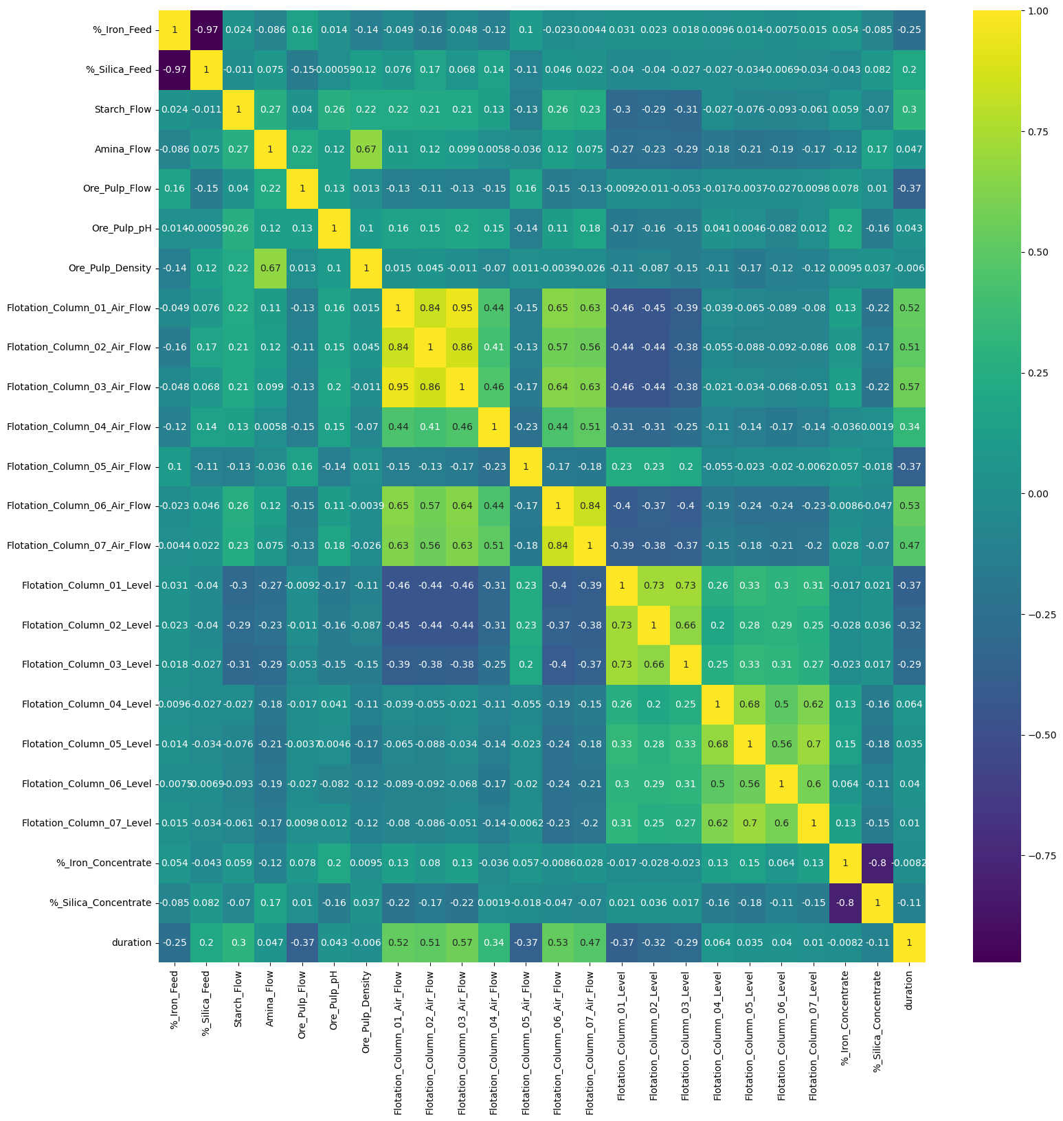
First you can tell the % of silica is negatively corelated to the % of iron concentrate, which makes sense since they are separately desired and undesired substance of the process, purity and impurity
Secondly, the airflow in column 1 is in general positively corelated to the airflow in column 2-7 except for column 5, which arise a potential doubt deserve diving deeper. Also we can tell the larger the airflow is, the lower the flotation level is in the responding column.
Thirdly, we can see from the correlation heat map that the ore pulp flow and starch flow barely have influence on the final product – % iron and % silica. on top of the fact that they both have positive corelation with the airflow measured in the columns, we can later verify the underlying collinearity by eigenvalue.

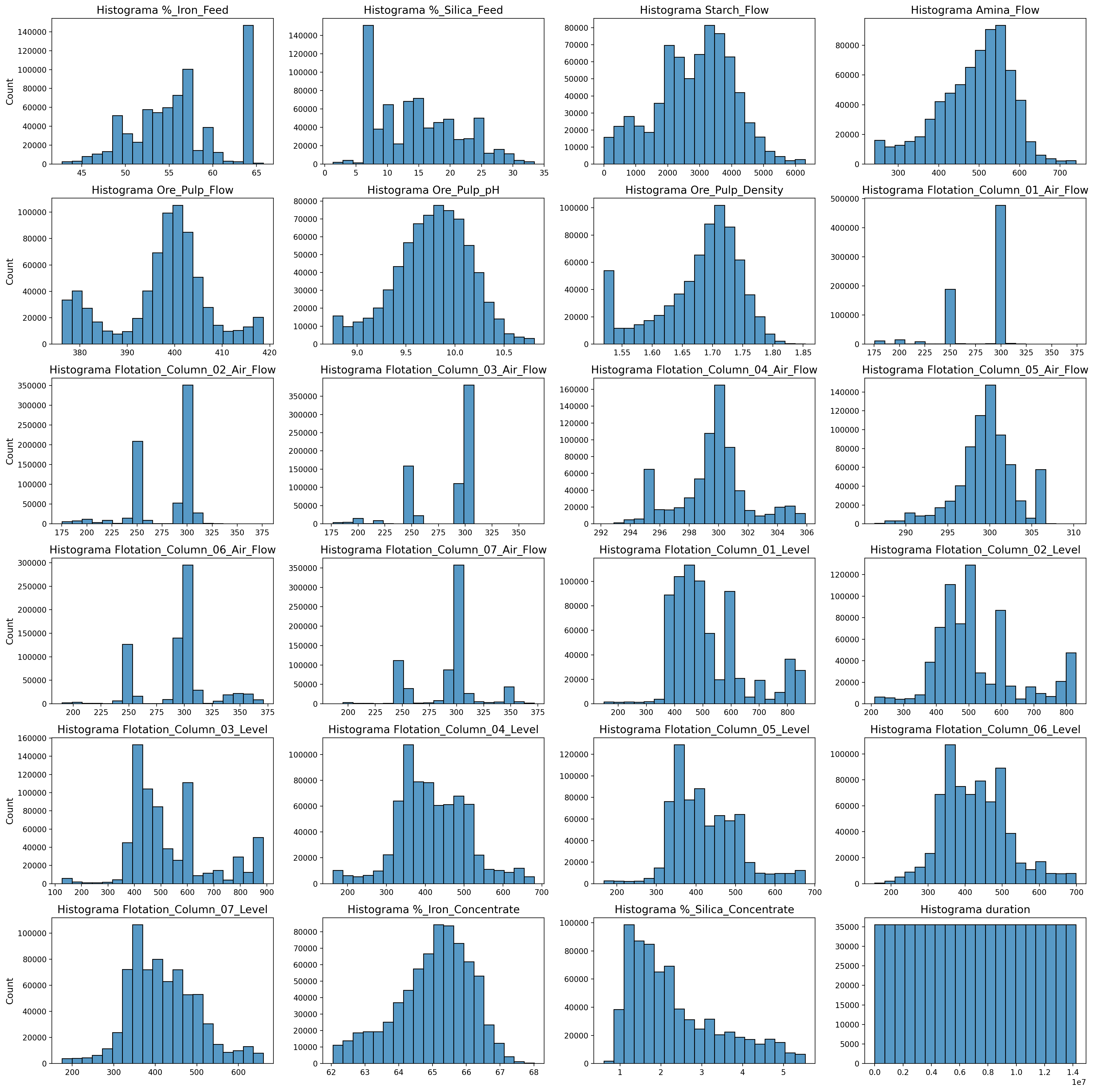
Feature Histogram-cross correlation and distribution

plt.figure(figsize=(20,20),dpi=200)
for i , n in enumerate(dt_df.columns.to_list()):
    plt.subplot(6,4,i+1)
    ax = sns.histplot(data=dt_df, x=n, kde=False, bins=20)#, multiple="stack")
    plt.title(f"Histograma {n}", fontdict={"fontsize":14})
    plt.xlabel("")
    plt.ylabel(ax.get_ylabel(), fontdict={"fontsize":12})
    if i not in [0,4,8,12,16,20,24]:
        plt.ylabel("")
    

plt.tight_layout();

png

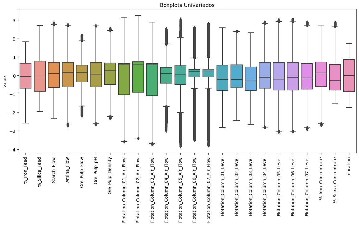
Feature Boxplot-distribution

scaler = StandardScaler()

z = pd.DataFrame(scaler.fit_transform(dt_df), columns=dt_df.columns, index=dt_df.index)
z = z.melt()

plt.figure(figsize=(14,6),dpi=100)
sns.boxplot(x=z["variable"], y=z["value"]);
plt.xticks(rotation=90);
plt.xlabel("");
plt.title("Boxplots Univariados");

png

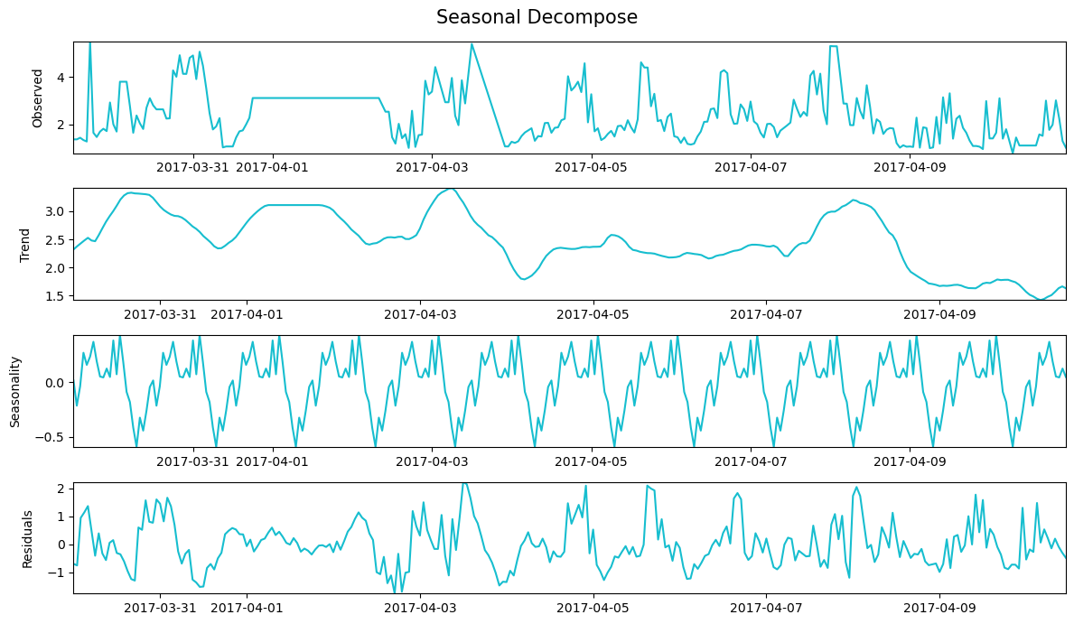
Timeseries lag trend

df_h = dt_df.resample('H').first()
df_h.index.names = ['Date']

result = seasonal_decompose(df_h["%_Silica_Concentrate"][:300])

def decompose_plot(result):

    fig,axes = plt.subplots(ncols=1,nrows=4,figsize=(12,7))

    axes[0].plot(result.observed.index, result.observed.values, color='tab:cyan')
    axes[0].set_ylabel("Observed",fontdict={"size":10,},labelpad=10)
    axes[0].set_xticks(axes[0].get_xticks(), rotation=45)

    axes[1].plot(result.trend.index, result.trend.values, color='tab:cyan')
    axes[1].set_ylabel("Trend",fontdict={"size":10,},labelpad=10)

    axes[2].plot(result.seasonal.index, result.seasonal.values, color='tab:cyan')
    axes[2].set_ylabel("Seasonality",fontdict={"size":10,},labelpad=10)

    axes[3].plot(result.resid.index, result.resid.values, color='tab:cyan')
    axes[3].set_ylabel("Residuals",fontdict={"size":10,},labelpad=10)
    
    for n in range(0,4):
        axes[n].autoscale(axis="both",tight=True)

    fig.suptitle("Seasonal Decompose",fontsize=15)
    plt.tight_layout()

decompose_plot(result)

png

Supervised TimeDiff Machine Learning

dt_df.columns

Index(['%_Iron_Feed', '%_Silica_Feed', 'Starch_Flow', 'Amina_Flow',
       'Ore_Pulp_Flow', 'Ore_Pulp_pH', 'Ore_Pulp_Density',
       'Flotation_Column_01_Air_Flow', 'Flotation_Column_02_Air_Flow',
       'Flotation_Column_03_Air_Flow', 'Flotation_Column_04_Air_Flow',
       'Flotation_Column_05_Air_Flow', 'Flotation_Column_06_Air_Flow',
       'Flotation_Column_07_Air_Flow', 'Flotation_Column_01_Level',
       'Flotation_Column_02_Level', 'Flotation_Column_03_Level',
       'Flotation_Column_04_Level', 'Flotation_Column_05_Level',
       'Flotation_Column_06_Level', 'Flotation_Column_07_Level',
       '%_Iron_Concentrate', '%_Silica_Concentrate', 'duration'],
      dtype='object')

list_cols = [col for col in dt_df.columns.to_list()]  # Use this if I want to include all explanatory variables.

list_cols.remove("%_Silica_Concentrate")
list_cols.remove("%_Iron_Concentrate")

# Resample the original df every 15 minutes.
df_15 = dt_df.resample("15min").first()
df_15 = df_15.drop("%_Iron_Concentrate", axis=1)

window_size = 3

# Taking advantage of the time factor, I add lagged explanatory variables at 15min, 30min, and 45min, respectively
# (these are the ones that were updated every 20s)

for col_name in list_cols:
    for i in range(window_size):
        df_15[f"{col_name} ({-15*(i+1)}mins)"] = df_15[f"{col_name}"].shift(periods=i+1)

# Resample from 15min to 1hour
df_h = df_15.resample('H').first()

# Here I change the name of my index.
df_h.index.names = ['Date']

# Add lagged values of the target variable as explanatory variables, lagged by 1, 2, and 3 hours respectively.
col_name = "%_Silica_Concentrate"
window_size = 3

for i in range(window_size):
    df_h[f"{col_name} ({-i-1}h)"] = df_h[f"{col_name}"].shift(periods=i+1)

# Make the target variable the first column.
x = df_h.columns.to_list()
x.remove("%_Silica_Concentrate")
x.insert(0, "%_Silica_Concentrate")
df_h = df_h[x]

df_h = df_h.dropna()  # Remove rows with missing values due to the shift().
df_h = df_h.astype("float32")  # Convert data to float32 for faster computation.

I create performance reporting functions for my model, a tracker to keep track of metrics, and also add a function to perform a time series split (where temporal order is respected).

Helper Functions

def plot_time_series(timesteps, values, start=0, end=None, label=None):#, #color="blue"):
    """
    Plots timesteps (a series of points in time) against values (a series of values across timesteps).

    Parameters
    ----------
    timesteps : array of timestep values
    values : array of values across time
    format : style of plot, default "."
    start : where to start the plot (setting a value will index from start of timesteps & values)
    end : where to end the plot (similar to start but for the end)
    label : label to show on plot about values, default None 
    """
  # Plot the series
    sns.lineplot(x=timesteps[start:end], y=values[start:end], label=label)
    plt.xlabel("Date")
    plt.ylabel("% Silica Concentrate")
    if label:
        plt.legend(fontsize=14) # make label bigger
    plt.grid(True)

def timeseries_report_model(y_test, model_preds, tracker_df="none", model_name="model_unknown", seasonality=1, naive=False):
    mae = round(mean_absolute_error(y_test, model_preds), 4)
    rmse = round(mean_squared_error(y_test, model_preds) ** 0.5, 4)
    mase = round(mean_absolute_scaled_error(y_test, model_preds, seasonality, naive),4)
    r2 = round(r2_score(y_test, model_preds), 4)
    mape = round(mean_absolute_percentage_error(y_test, model_preds), 4)

    print("MAE: ", mae)
    print("RMSE :", rmse)
    print("MASE :", mase)
    print("R2 :", r2)
    print("MAPE :", mape)

    if isinstance(tracker_df, pd.core.frame.DataFrame):
        tracker_df.loc[tracker_df.shape[0]] = [
            model_name, mae, rmse, mase, r2, mape]
    else:
        pass

LSTM model

# Make the train/test splits
def make_train_test_splits(windows, labels, test_split=0.2):
    """
    Splits matching pairs of winodws and labels into train and test splits.
    """
    split_size = int(len(windows) * (1-test_split)) # this will default to 80% train/20% test
    train_windows = windows[:split_size]
    train_labels = labels[:split_size]
    test_windows = windows[split_size:]
    test_labels = labels[split_size:]
    return train_windows, test_windows, train_labels, test_labels

df_forecast = df_h.copy()
df_forecast.shape

(3946, 92)

tracker = timeseries_models_tracker_df()

X = df_forecast.drop("%_Silica_Concentrate", axis=1)
y = df_forecast["%_Silica_Concentrate"]

train_windows, test_windows, train_labels, test_labels = make_train_test_splits(X,y,test_split=0.1)
len(train_windows), len(test_windows), len(train_labels), len(test_labels)

(3551, 395, 3551, 395)

warnings.filterwarnings("ignore")
def objective(trial, X,y):


    
    param_grid = {
        "random_state": 123,
        "verbosity": -1,
        "boosting_type": trial.suggest_categorical("boosting_type", ['gbdt']),#,"goss"]),
        "device_type": trial.suggest_categorical("device_type", ['cpu']),
        "n_estimators": trial.suggest_int("n_estimators", 25, 10000,step=100), #for large datasets this should be very high
        "learning_rate": trial.suggest_float("learning_rate", 0.001, 0.3),
        "num_leaves": trial.suggest_int("num_leaves", 10, 190), # Also change this for large datasets, should be small to avoid overfitting
        "max_depth": trial.suggest_int("max_depth", 2, 80),
        "min_child_samples": trial.suggest_int("min_child_samples", 10, 800, step=20), #modify this for large datasets, causes overfittin if too low
        "reg_alpha": trial.suggest_float("reg_alpha", 0.0001, 1000, log=True),
        "reg_lambda": trial.suggest_float("reg_lambda", 0.0001, 1000, log=True),
        #"min_split_gain": trial.suggest_float("min_split_gain", 0, 3),
        "subsample": trial.suggest_float("subsample", 0.05, 1, step=0.05),
        "subsample_freq": trial.suggest_categorical("subsample_freq", [0,1]), #[0,1] bagging
        "colsample_bytree": trial.suggest_float("colsample_bytree", 0.3, 1, step=0.1),
    }
    
    #min_data_in_leaf # min_child_samples
    
    # RMSE (Root Mean Squared Error)
    def rmse(y_val,y_pred):
        is_higher_better = False
        name = "rmse"
        value = mean_squared_error(y_val,y_pred, squared=False)
        return name, value, is_higher_better
    
    cv_scores = np.empty(5)
    
    tscv = TimeSeriesSplit(n_splits=5, max_train_size=None)
    
    for idx , (train_index, val_index) in enumerate(tscv.split(X)):
        X_train, X_val = X.iloc[train_index], X.iloc[val_index]
        y_train, y_val = y.iloc[train_index], y.iloc[val_index]
        

        model = LGBMRegressor(objective="regression", silent=True,**param_grid)
        model.fit(
            X_train,
            y_train,
            eval_set=[(X_val, y_val)],
            eval_metric=rmse,
            early_stopping_rounds=100,
            categorical_feature="auto",   # cat_idx, #specifiy categorial features.
            callbacks=[LightGBMPruningCallback(trial, "l2", report_interval=20)],  # Add a pruning callback
            verbose=0)

        preds =  model.predict(X_val)
        rmse = mean_squared_error(y_val,preds, squared=False)

        cv_scores[idx] = rmse

    
    return np.mean(cv_scores)

study = optuna.create_study(direction="minimize", study_name="LGBM Regressor",sampler=TPESampler(),
                            pruner=optuna.pruners.PercentilePruner(50, n_startup_trials=5, n_warmup_steps=50))

#study.enqueue_trial(try_this_first)
func = lambda trial: objective(trial, train_windows, train_labels)
study.optimize(func, n_trials=100)

[32m[I 2023-04-14 20:06:45,615][0m A new study created in memory with name: LGBM Regressor[0m
[32m[I 2023-04-14 20:06:46,696][0m Trial 0 finished with value: 0.8109004958352836 and parameters: {'boosting_type': 'gbdt', 'device_type': 'cpu', 'n_estimators': 8325, 'learning_rate': 0.2136801933659405, 'num_leaves': 122, 'max_depth': 24, 'min_child_samples': 290, 'reg_alpha': 0.4089594656291566, 'reg_lambda': 233.41962530839834, 'subsample': 0.55, 'subsample_freq': 1, 'colsample_bytree': 0.5}. Best is trial 0 with value: 0.8109004958352836.[0m
[32m[I 2023-04-14 20:06:47,790][0m Trial 1 finished with value: 0.8149075483133782 and parameters: {'boosting_type': 'gbdt', 'device_type': 'cpu', 'n_estimators': 2625, 'learning_rate': 0.20374443271553472, 'num_leaves': 24, 'max_depth': 65, 'min_child_samples': 550, 'reg_alpha': 0.00011716269934726968, 'reg_lambda': 0.005714841791728027, 'subsample': 0.45, 'subsample_freq': 0, 'colsample_bytree': 0.8}. Best is trial 0 with value: 0.8109004958352836.[0m
......
[32m[I 2023-04-14 20:08:36,711][0m Trial 99 finished with value: 0.718496606821031 and parameters: {'boosting_type': 'gbdt', 'device_type': 'cpu', 'n_estimators': 3425, 'learning_rate': 0.25476699329382246, 'num_leaves': 78, 'max_depth': 44, 'min_child_samples': 30, 'reg_alpha': 0.006442917820858156, 'reg_lambda': 0.9818132921273436, 'subsample': 0.45, 'subsample_freq': 1, 'colsample_bytree': 0.8}. Best is trial 71 with value: 0.7022349235029833.[0m

# Train again using the optimized hyperparameters
params = study.best_params
model = LGBMRegressor(objective="regression",random_state=123,**params)
model.fit(train_windows, train_labels)

LGBMRegressor(colsample_bytree=0.8, device_type='cpu',
              learning_rate=0.2514458173401127, max_depth=48,
              min_child_samples=90, n_estimators=2125, num_leaves=128,
              objective='regression', random_state=123,
              reg_alpha=0.0042343839479169615, reg_lambda=8.01369798587411,
              subsample=0.6500000000000001, subsample_freq=1)

preds = model.predict(test_windows)
timeseries_report_model(test_labels, preds, tracker, model_name="Experiment , LightGBM",
                        seasonality=1, naive=False)

MAE:  0.6045
RMSE : 0.8177
MASE : 1.1928
R2 : 0.5233
MAPE : 0.2752

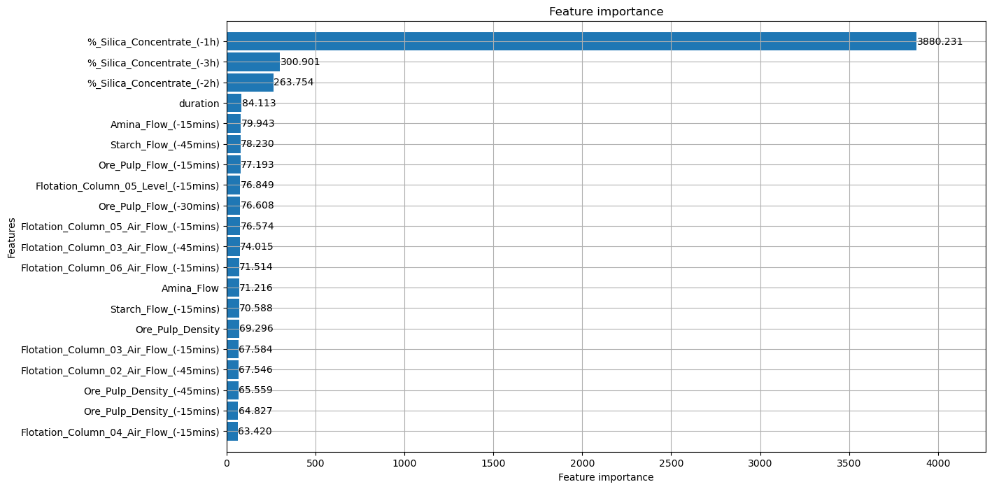
plot_importance(model, max_num_features = 20, height=.9, importance_type="gain", figsize=(14,8));

png

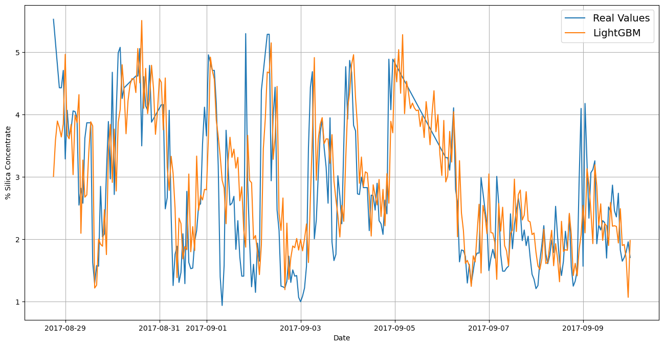
plt.figure(figsize=(16,8),dpi=100)
plot_time_series(test_labels.index, test_labels, label="Real Values", start=100)
plot_time_series(test_labels.index, preds,label="LightGBM", start=100)

png